Simulate Responses From merMod Object — simulate.merMod • lme4

Simulate responses from a "merMod" fitted model object, i.e., from the model represented by it.

Usage

# S3 method for class 'merMod'
simulate(object, nsim = 1, seed = NULL,
   use.u = FALSE, re.form = NA,
   newdata=NULL, newparams=NULL, family=NULL, cluster.rand=rnorm,
   allow.new.levels = FALSE, na.action = na.pass, ...)

.simulateFun(object, nsim = 1, seed = NULL, use.u = FALSE,
             re.form = NA,
             newdata=NULL, newparams=NULL,
             formula=NULL, family=NULL, 
             cluster.rand=rnorm,
             weights=NULL, offset=NULL,
             allow.new.levels = FALSE, na.action = na.pass,
             cond.sim = TRUE, ...)

Arguments

object: (for simulate.merMod) a fitted model object or (for simulate.formula) a (one-sided) mixed model formula, as described for lmer.
nsim: positive integer scalar - the number of responses to simulate.
seed: an optional seed to be used in set.seed immediately before the simulation so as to generate a reproducible sample.
use.u: (logical) if TRUE, generate a simulation conditional on the current random-effects estimates; if FALSE generate new Normally distributed random-effects values. (Redundant with re.form, which is preferred: TRUE corresponds to re.form = NULL (condition on all random effects), while FALSE corresponds to re.form = ~0 (condition on none of the random effects).)
re.form: formula for random effects to condition on. If NULL, condition on all random effects; if NA or ~0, condition on no random effects. See Details.
newdata: data frame for which to evaluate predictions.
newparams: new parameters to use in evaluating predictions, specified as in the start parameter for lmer or glmer – a list with components theta and beta and (for LMMs or GLMMs that estimate a scale parameter) sigma
formula: a (one-sided) mixed model formula, as described for lmer.
family: a GLM family, as in glmer.
cluster.rand: Function that generates standardized random cluster effects. The function takes one argument, the number of random values to generate.
weights: prior weights, as in lmer or glmer.
offset: offset, as in glmer.
allow.new.levels: (logical) if FALSE (default), then any new levels (or NA values) detected in newdata will trigger an error; if TRUE, then the prediction will use the unconditional (population-level) values for data with previously unobserved levels (or NAs).
na.action: what to do with NA values in new data: see na.fail
cond.sim: (experimental) simulate the conditional distribution? if FALSE, simulate only random effects; do not simulate from the conditional distribution, rather return the predicted group-level values
...: optional additional arguments (none are used in .simulateFormula)

Details

ordinarily simulate is used to generate new values from an existing, fitted model (merMod object): however, if formula, newdata, and newparams are specified, simulate generates the appropriate model structure to simulate from. formula must be a one-sided formula (i.e. with an empty left-hand side); in general, if f is a two-sided formula, f[-2] can be used to drop the LHS.
The re.form argument allows the user to specify how the random effects are incorporated in the simulation. All of the random effects terms included in re.form will be conditioned on - that is, the conditional modes of those random effects will be included in the deterministic part of the simulation. (If new levels are used (and allow.new.levels is TRUE), the conditional modes for these levels will be set to the population mode, i.e. values of zero will be used for the random effects.) Conversely, the random effect terms that are not included in re.form will be simulated from - that is, new values will be chosen for each group based on the estimated random-effects variances. The default behaviour (using re.form=NA) is to condition on none of the random effects, simulating new values for all of the random effects.
For Gaussian fits, sigma specifies the residual standard deviation; for Gamma fits, it specifies the shape parameter (the rate parameter for each observation i is calculated as shape/mean(i)). For negative binomial fits, the overdispersion parameter is specified via the family, e.g. simulate(..., family=negative.binomial(theta=1.5)).
For binomial models, simulate.formula looks for the binomial size first in the weights argument (if it's supplied), second from the left-hand side of the formula (if the formula has been specified in success/failure form), and defaults to 1 if neither of those have been supplied. Simulated responses will be given as proportions, unless the supplied formula has a matrix-valued left-hand side, in which case they will be given in matrix form. If a left-hand side is given, variables in that expression must be available in newdata.
For negative binomial models, use the negative.binomial family (from the MASS package) and specify the overdispersion parameter via the theta (sic) parameter of the family function, e.g. simulate(...,family=negative.binomial(theta=1)) to simulate from a geometric distribution (negative binomial with overdispersion parameter 1).
cluster.rand allows one to test effects of departures from normality for the distribution of cluster random effects, for example by using a heavy-tailed distribution or a mixture distribution. One can also use a truncated normal to investigate true or false flagging rates; in that case the generated effects will not have a mean of 0 and standard deviation of 1; they are still considered standardized in that the simulation will multiply them by the estimated standard deviation of the cluster random effects.

Examples

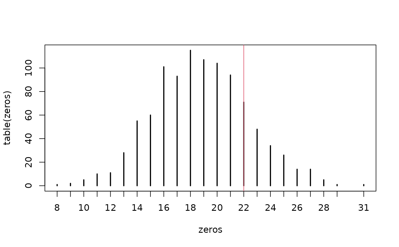
## test whether fitted models are consistent with the
##  observed number of zeros in CBPP data set:
gm1 <- glmer(cbind(incidence, size - incidence) ~ period + (1 | herd),
             data = cbpp, family = binomial)
gg <- simulate(gm1,1000)
zeros <- sapply(gg,function(x) sum(x[,"incidence"]==0))
plot(table(zeros))
abline(v=sum(cbpp$incidence==0),col=2)

##
## simulate from a non-fitted model; in this case we are just
## replicating the previous model, but starting from scratch
params <- list(theta=0.5,beta=c(2,-1,-2,-3))
simdat <- with(cbpp,expand.grid(herd=levels(herd),period=factor(1:4)))
simdat$size <- 15
simdat$incidence <- sample(0:1,size=nrow(simdat),replace=TRUE)
form <- formula(gm1)[-2]  ## RHS of equation only
simulate(form,newdata=simdat,family=binomial,
    newparams=params)
#>    sim_1
#> 1      1
#> 2      1
#> 3      0
#> 4      1
#> 5      1
#> 6      1
#> 7      1
#> 8      1
#> 9      1
#> 10     1
#> 11     1
#> 12     0
#> 13     1
#> 14     1
#> 15     1
#> 16     0
#> 17     0
#> 18     0
#> 19     1
#> 20     0
#> 21     1
#> 22     0
#> 23     1
#> 24     1
#> 25     1
#> 26     1
#> 27     1
#> 28     0
#> 29     1
#> 30     1
#> 31     0
#> 32     0
#> 33     0
#> 34     0
#> 35     0
#> 36     0
#> 37     1
#> 38     0
#> 39     1
#> 40     1
#> 41     1
#> 42     1
#> 43     0
#> 44     1
#> 45     1
#> 46     0
#> 47     0
#> 48     0
#> 49     0
#> 50     1
#> 51     0
#> 52     0
#> 53     1
#> 54     1
#> 55     0
#> 56     0
#> 57     0
#> 58     0
#> 59     0
#> 60     0
## simulate from negative binomial distribution instead
simulate(form,newdata=simdat,family=negative.binomial(theta=2.5),
    newparams=params)
#>    sim_1
#> 1     11
#> 2      2
#> 3      7
#> 4      6
#> 5     18
#> 6      8
#> 7     47
#> 8     11
#> 9      6
#> 10    25
#> 11     7
#> 12     7
#> 13     1
#> 14    14
#> 15     2
#> 16     9
#> 17     1
#> 18     0
#> 19     1
#> 20     0
#> 21     3
#> 22     1
#> 23     2
#> 24     2
#> 25     9
#> 26     2
#> 27     7
#> 28     0
#> 29     3
#> 30     6
#> 31     5
#> 32     1
#> 33     0
#> 34     0
#> 35     0
#> 36     0
#> 37     9
#> 38     1
#> 39     0
#> 40     1
#> 41     3
#> 42     0
#> 43     1
#> 44     6
#> 45     1
#> 46     1
#> 47     1
#> 48     1
#> 49     0
#> 50     0
#> 51     0
#> 52     2
#> 53     0
#> 54     0
#> 55     0
#> 56     0
#> 57     0
#> 58     0
#> 59     1
#> 60     0

Simulate Responses From `merMod` Object

Usage

Arguments

See also

Details

Examples