Fitting Generalized Linear Mixed-Effects Models

Fit a generalized linear mixed-effects model (GLMM). Both fixed effects and random effects are specified via the model formula.

Usage

glmer(formula, data = NULL, family = gaussian
    , control = glmerControl()
    , start = NULL
    , verbose = 0L
    , nAGQ = 1L
    , subset, weights, na.action, offset, contrasts = NULL
    , mustart, etastart
    , devFunOnly = FALSE)

Arguments

formula: a two-sided linear formula object describing both the fixed-effects and random-effects part of the model, with the response on the left of a ~ operator and the terms, separated by + operators, on the right. Random-effects terms are distinguished by vertical bars ("|") separating expressions for design matrices from grouping factors.
data: an optional data frame containing the variables named in formula. By default the variables are taken from the environment from which lmer is called. While data is optional, the package authors strongly recommend its use, especially when later applying methods such as update and drop1 to the fitted model (such methods are not guaranteed to work properly if data is omitted). If data is omitted, variables will be taken from the environment of formula (if specified as a formula) or from the parent frame (if specified as a character vector).
family: a GLM family, see glm and family.
control: a list (of correct class, resulting from lmerControl() or glmerControl() respectively) containing control parameters, including the nonlinear optimizer to be used and parameters to be passed through to the nonlinear optimizer, see the *lmerControl documentation for details.
start: a named list of starting values for the parameters in the model, or a numeric vector. A numeric start argument will be used as the starting value of theta. If start is a list, the theta element (a numeric vector) is used as the starting value for the first optimization step (default=1 for diagonal elements and 0 for off-diagonal elements of the lower Cholesky factor); the fitted value of theta from the first step, plus start[["fixef"]], are used as starting values for the second optimization step. If start has both fixef and theta elements, the first optimization step is skipped. For more details or finer control of optimization, see modular.
verbose: integer scalar. If > 0 verbose output is generated during the optimization of the parameter estimates. If > 1 verbose output is generated during the individual penalized iteratively reweighted least squares (PIRLS) steps.
nAGQ: integer scalar - the number of points per axis for evaluating the adaptive Gauss-Hermite approximation to the log-likelihood. Defaults to 1, corresponding to the Laplace approximation. Values greater than 1 produce greater accuracy in the evaluation of the log-likelihood at the expense of speed. A value of zero uses a faster but less exact form of parameter estimation for GLMMs by optimizing the random effects and the fixed-effects coefficients in the penalized iteratively reweighted least squares step. (See Details.)
subset: an optional expression indicating the subset of the rows of data that should be used in the fit. This can be a logical vector, or a numeric vector indicating which observation numbers are to be included, or a character vector of the row names to be included. All observations are included by default.
weights: an optional vector of ‘prior weights’ to be used in the fitting process. Should be NULL or a numeric vector.
na.action: a function that indicates what should happen when the data contain NAs. The default action (na.omit, inherited from the ‘factory fresh’ value of getOption("na.action")) strips any observations with any missing values in any variables.
offset: this can be used to specify an a priori known component to be included in the linear predictor during fitting. This should be NULL or a numeric vector of length equal to the number of cases. One or more offset terms can be included in the formula instead or as well, and if more than one is specified their sum is used. See model.offset.
contrasts: an optional list. See the contrasts.arg of model.matrix.default.
mustart: optional starting values on the scale of the conditional mean, as in glm; see there for details.
etastart: optional starting values on the scale of the unbounded predictor as in glm; see there for details.
devFunOnly: logical - return only the deviance evaluation function. Note that because the deviance function operates on variables stored in its environment, it may not return exactly the same values on subsequent calls (but the results should always be within machine tolerance).

Value

An object of class merMod (more specifically, an object of subclass glmerMod) for which many methods are available (e.g. methods(class="merMod"))

Note

In earlier version of the lme4 package, a method argument was used. Its functionality has been replaced by the nAGQ argument.

Details

Fit a generalized linear mixed model, which incorporates both fixed-effects parameters and random effects in a linear predictor, via maximum likelihood. The linear predictor is related to the conditional mean of the response through the inverse link function defined in the GLM family.

The expression for the likelihood of a mixed-effects model is an integral over the random effects space. For a linear mixed-effects model (LMM), as fit by lmer, this integral can be evaluated exactly. For a GLMM the integral must be approximated. The most reliable approximation for GLMMs is adaptive Gauss-Hermite quadrature, at present implemented only for models with a single scalar random effect. The nAGQ argument controls the number of nodes in the quadrature formula. A model with a single, scalar random-effects term could reasonably use up to 25 quadrature points per scalar integral.

Examples

## generalized linear mixed model
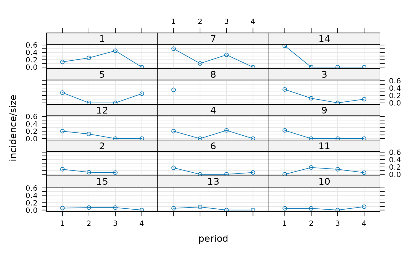
library(lattice)
xyplot(incidence/size ~ period|herd, cbpp, type=c('g','p','l'),
       layout=c(3,5), index.cond = function(x,y)max(y))

(gm1 <- glmer(cbind(incidence, size - incidence) ~ period + (1 | herd),
              data = cbpp, family = binomial))
#> Generalized linear mixed model fit by maximum likelihood (Laplace
#>   Approximation) [glmerMod]
#>  Family: binomial  ( logit )
#> Formula: cbind(incidence, size - incidence) ~ period + (1 | herd)
#>    Data: cbpp
#>       AIC       BIC    logLik -2*log(L)  df.resid 
#>  194.0531  204.1799  -92.0266  184.0531        51 
#> Random effects:
#>  Groups Name        Std.Dev.
#>  herd   (Intercept) 0.6421  
#> Number of obs: 56, groups:  herd, 15
#> Fixed Effects:
#> (Intercept)      period2      period3      period4  
#>     -1.3983      -0.9919      -1.1282      -1.5797  
## using nAGQ=0 only gets close to the optimum
(gm1a <- glmer(cbind(incidence, size - incidence) ~ period + (1 | herd),
               cbpp, binomial, nAGQ = 0))
#> Generalized linear mixed model fit by maximum likelihood (Adaptive
#>   Gauss-Hermite Quadrature, nAGQ = 0) [glmerMod]
#>  Family: binomial  ( logit )
#> Formula: cbind(incidence, size - incidence) ~ period + (1 | herd)
#>    Data: cbpp
#>       AIC       BIC    logLik -2*log(L)  df.resid 
#>  194.1087  204.2355  -92.0543  184.1087        51 
#> Random effects:
#>  Groups Name        Std.Dev.
#>  herd   (Intercept) 0.6418  
#> Number of obs: 56, groups:  herd, 15
#> Fixed Effects:
#> (Intercept)      period2      period3      period4  
#>     -1.3605      -0.9762      -1.1111      -1.5597  
## using  nAGQ = 9  provides a better evaluation of the deviance
## Currently the internal calculations use the sum of deviance residuals,
## which is not directly comparable with the nAGQ=0 or nAGQ=1 result.
## 'verbose = 1' monitors iteratin a bit; (verbose = 2 does more):
(gm1a <- glmer(cbind(incidence, size - incidence) ~ period + (1 | herd),
               cbpp, binomial, verbose = 1, nAGQ = 9))
#> start par. =  1 fn =  186.7231 
#> At return
#> eval:  18 fn:      184.10869 par: 0.641839
#> (NM) 20: f = 100.035 at   0.65834  -1.40366 -0.973379  -1.12553  -1.51926
#> (NM) 40: f = 100.012 at  0.650182  -1.39827 -0.993156  -1.11768  -1.57305
#> (NM) 60: f = 100.011 at  0.649102  -1.39735 -0.999034  -1.13415  -1.57634
#> (NM) 80: f = 100.01 at  0.647402  -1.39987 -0.987353  -1.12767  -1.57516
#> (NM) 100: f = 100.01 at   0.64823      -1.4 -0.991134  -1.12755  -1.58048
#> (NM) 120: f = 100.01 at  0.647543  -1.39916 -0.991869  -1.12839  -1.57993
#> (NM) 140: f = 100.01 at  0.647452  -1.39935 -0.991366  -1.12764  -1.57936
#> (NM) 160: f = 100.01 at  0.647519  -1.39925 -0.991348  -1.12784  -1.57948
#> (NM) 180: f = 100.01 at  0.647513  -1.39924 -0.991381  -1.12783  -1.57947
#> Generalized linear mixed model fit by maximum likelihood (Adaptive
#>   Gauss-Hermite Quadrature, nAGQ = 9) [glmerMod]
#>  Family: binomial  ( logit )
#> Formula: cbind(incidence, size - incidence) ~ period + (1 | herd)
#>    Data: cbpp
#>       AIC       BIC    logLik -2*log(L)  df.resid 
#>  110.0100  120.1368  -50.0050  100.0100        51 
#> Random effects:
#>  Groups Name        Std.Dev.
#>  herd   (Intercept) 0.6475  
#> Number of obs: 56, groups:  herd, 15
#> Fixed Effects:
#> (Intercept)      period2      period3      period4  
#>     -1.3992      -0.9914      -1.1278      -1.5795  

## GLMM with individual-level variability (accounting for overdispersion)
## For this data set the model is the same as one allowing for a period:herd
## interaction, which the plot indicates could be needed.
cbpp$obs <- 1:nrow(cbpp)
(gm2 <- glmer(cbind(incidence, size - incidence) ~ period +
    (1 | herd) +  (1|obs),
              family = binomial, data = cbpp))
#> Generalized linear mixed model fit by maximum likelihood (Laplace
#>   Approximation) [glmerMod]
#>  Family: binomial  ( logit )
#> Formula: cbind(incidence, size - incidence) ~ period + (1 | herd) + (1 |  
#>     obs)
#>    Data: cbpp
#>       AIC       BIC    logLik -2*log(L)  df.resid 
#>  186.6383  198.7904  -87.3192  174.6383        50 
#> Random effects:
#>  Groups Name        Std.Dev.
#>  obs    (Intercept) 0.8911  
#>  herd   (Intercept) 0.1840  
#> Number of obs: 56, groups:  obs, 56; herd, 15
#> Fixed Effects:
#> (Intercept)      period2      period3      period4  
#>      -1.500       -1.226       -1.329       -1.866  
anova(gm1,gm2)
#> Data: cbpp
#> Models:
#> gm1: cbind(incidence, size - incidence) ~ period + (1 | herd)
#> gm2: cbind(incidence, size - incidence) ~ period + (1 | herd) + (1 | obs)
#>     npar    AIC    BIC  logLik -2*log(L)  Chisq Df Pr(>Chisq)   
#> gm1    5 194.05 204.18 -92.027    184.05                        
#> gm2    6 186.64 198.79 -87.319    174.64 9.4148  1   0.002152 **
#> ---
#> Signif. codes:  0 ‘***’ 0.001 ‘**’ 0.01 ‘*’ 0.05 ‘.’ 0.1 ‘ ’ 1

## glmer and glm log-likelihoods are consistent
gm1Devfun <- update(gm1,devFunOnly=TRUE)
gm0 <- glm(cbind(incidence, size - incidence) ~ period,
           family = binomial, data = cbpp)
## evaluate GLMM deviance at RE variance=theta=0, beta=(GLM coeffs)
gm1Dev0 <- gm1Devfun(c(0,coef(gm0)))
## compare
stopifnot(all.equal(gm1Dev0,c(-2*logLik(gm0))))
## the toenail oncholysis data from Backer et al 1998
## these data are notoriously difficult to fit
if (FALSE) { # \dontrun{
if (require("HSAUR3")) {
    gm2 <- glmer(outcome~treatment*visit+(1|patientID),
                 data=toenail,
                 family=binomial,nAGQ=20)
}
} # }