Diagnostic Plots for 'merMod' Fits

diagnostic plots for merMod fits

Usage

# S3 method for class 'merMod'
plot(x,
     form = resid(., type = "pearson") ~ fitted(.), abline,
     id = NULL, idLabels = NULL, grid, ...)
# S3 method for class 'merMod'
qqmath(x, data = NULL, id = NULL, idLabels = NULL, ...)

Arguments

x: a fitted [ng]lmer model
form: an optional formula specifying the desired type of plot. Any variable present in the original data frame used to obtain x can be referenced. In addition, x itself can be referenced in the formula using the symbol ".". Conditional expressions on the right of a | operator can be used to define separate panels in a lattice display. Default is resid(., type = "pearson") ~ fitted(.), corresponding to a plot of the standardized residuals versus fitted values.
abline: an optional numeric value, or numeric vector of length two. If given as a single value, a horizontal line will be added to the plot at that coordinate; else, if given as a vector, its values are used as the intercept and slope for a line added to the plot. If missing, no lines are added to the plot.
id: an optional numeric value, or one-sided formula. If given as a value, it is used as a significance level for a two-sided outlier test for the standardized, or normalized residuals. Observations with absolute standardized (normalized) residuals greater than the \(1-value/2\) quantile of the standard normal distribution are identified in the plot using idLabels. If given as a one-sided formula, its right hand side must evaluate to a logical, integer, or character vector which is used to identify observations in the plot. If missing, no observations are identified.
idLabels: an optional vector, or one-sided formula. If given as a vector, it is converted to character and used to label the observations identified according to id. If given as a vector, it is converted to character and used to label the observations identified according to id. If given as a one-sided formula, its right hand side must evaluate to a vector which is converted to character and used to label the identified observations. Default is the interaction of all the grouping variables in the data frame. The special formula idLabels=~.obs will label the observations according to observation number.
data: ignored: required for S3 method compatibility
grid: an optional logical value indicating whether a grid should be added to plot. Default depends on the type of lattice plot used: if xyplot defaults to TRUE, else defaults to FALSE.
...: optional arguments passed to the lattice plot function.

Details

Diagnostic plots for the linear mixed-effects fit are obtained. The form argument gives considerable flexibility in the type of plot specification. A conditioning expression (on the right side of a | operator) always implies that different panels are used for each level of the conditioning factor, according to a lattice display. If form is a one-sided formula, histograms of the variable on the right hand side of the formula, before a | operator, are displayed (the lattice function histogram is used). If form is two-sided and both its left and right hand side variables are numeric, scatter plots are displayed (the lattice function xyplot is used). Finally, if form is two-sided and its left had side variable is a factor, box-plots of the right hand side variable by the levels of the left hand side variable are displayed (the lattice function bwplot is used).

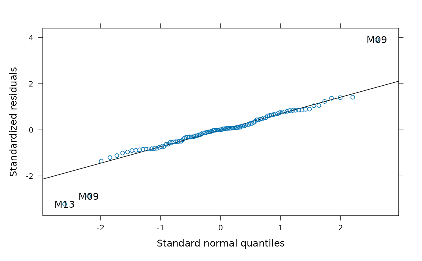
qqmath produces a Q-Q plot of the residuals (see qqmath.ranef.mer for Q-Q plots of the conditional mode values).

Author

original version in nlme package by Jose Pinheiro and Douglas Bates.

Examples

data(Orthodont,package="nlme")
fm1 <- lmer(distance ~ age + (age|Subject), data=Orthodont)
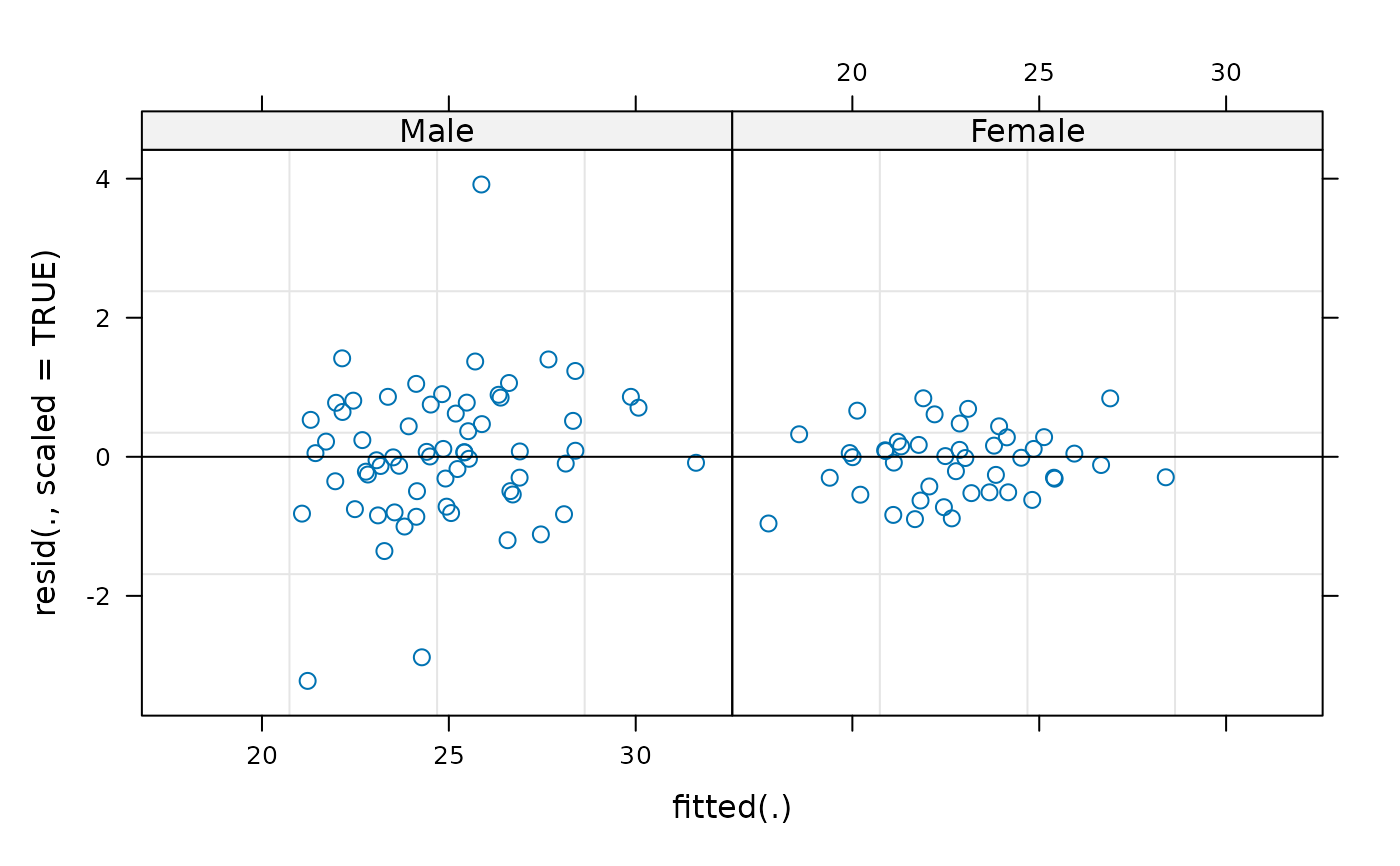
## standardized residuals versus fitted values by gender
plot(fm1, resid(., scaled=TRUE) ~ fitted(.) | Sex, abline = 0)

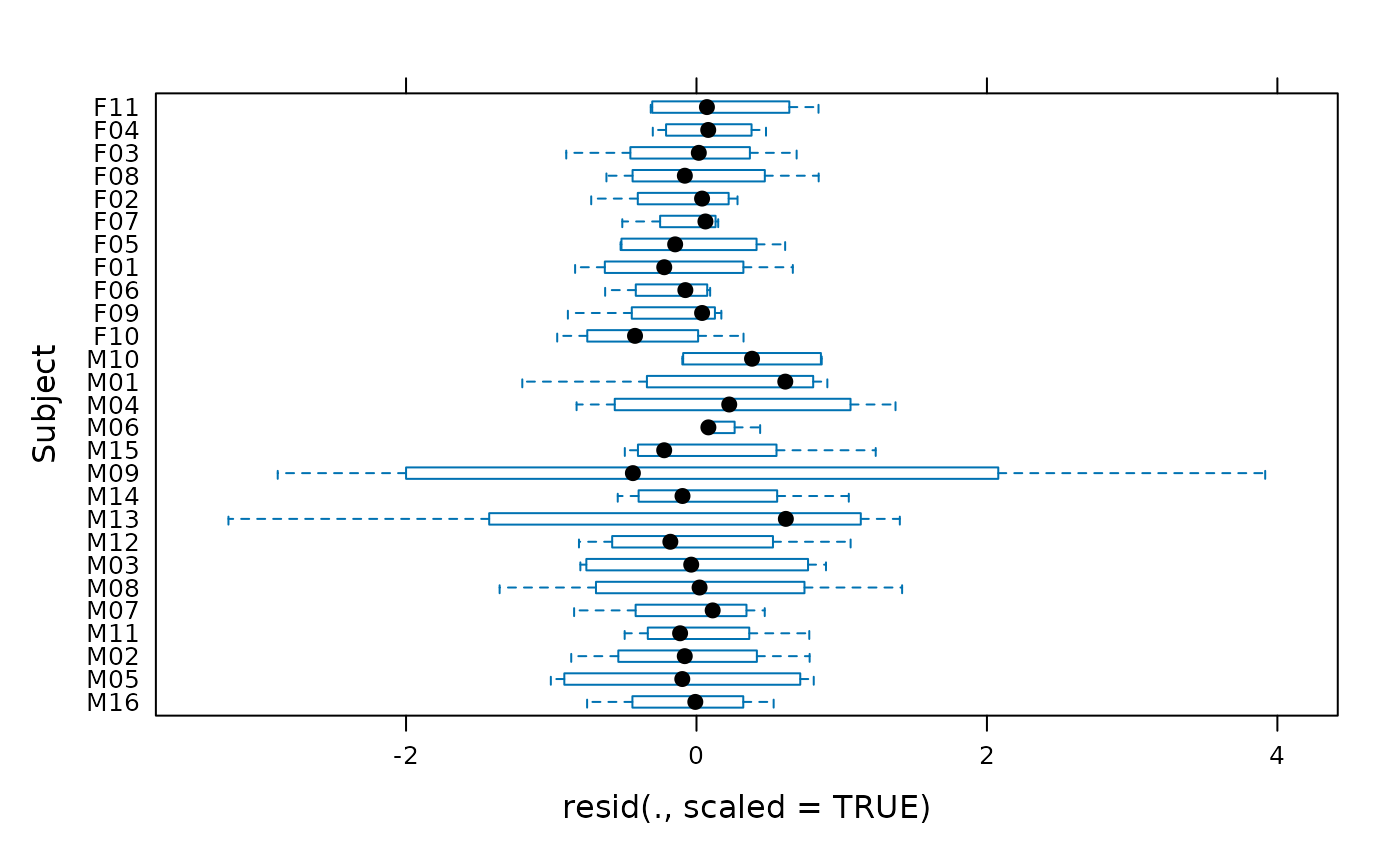
## box-plots of residuals by Subject
plot(fm1, Subject ~ resid(., scaled=TRUE))

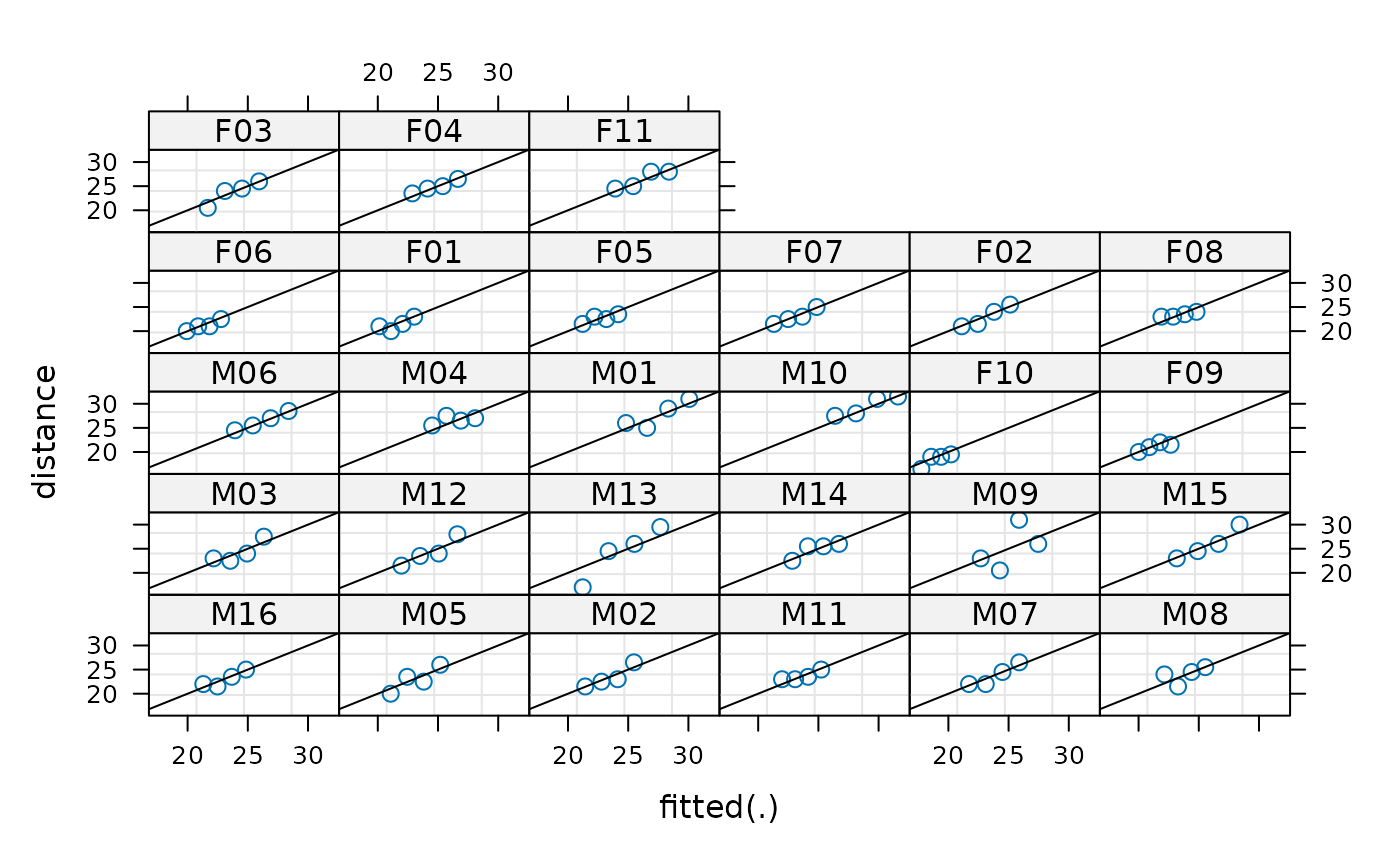
## observed versus fitted values by Subject
plot(fm1, distance ~ fitted(.) | Subject, abline = c(0,1))

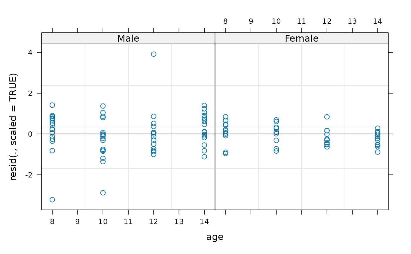
## residuals by age, separated by Subject
plot(fm1, resid(., scaled=TRUE) ~ age | Sex, abline = 0)

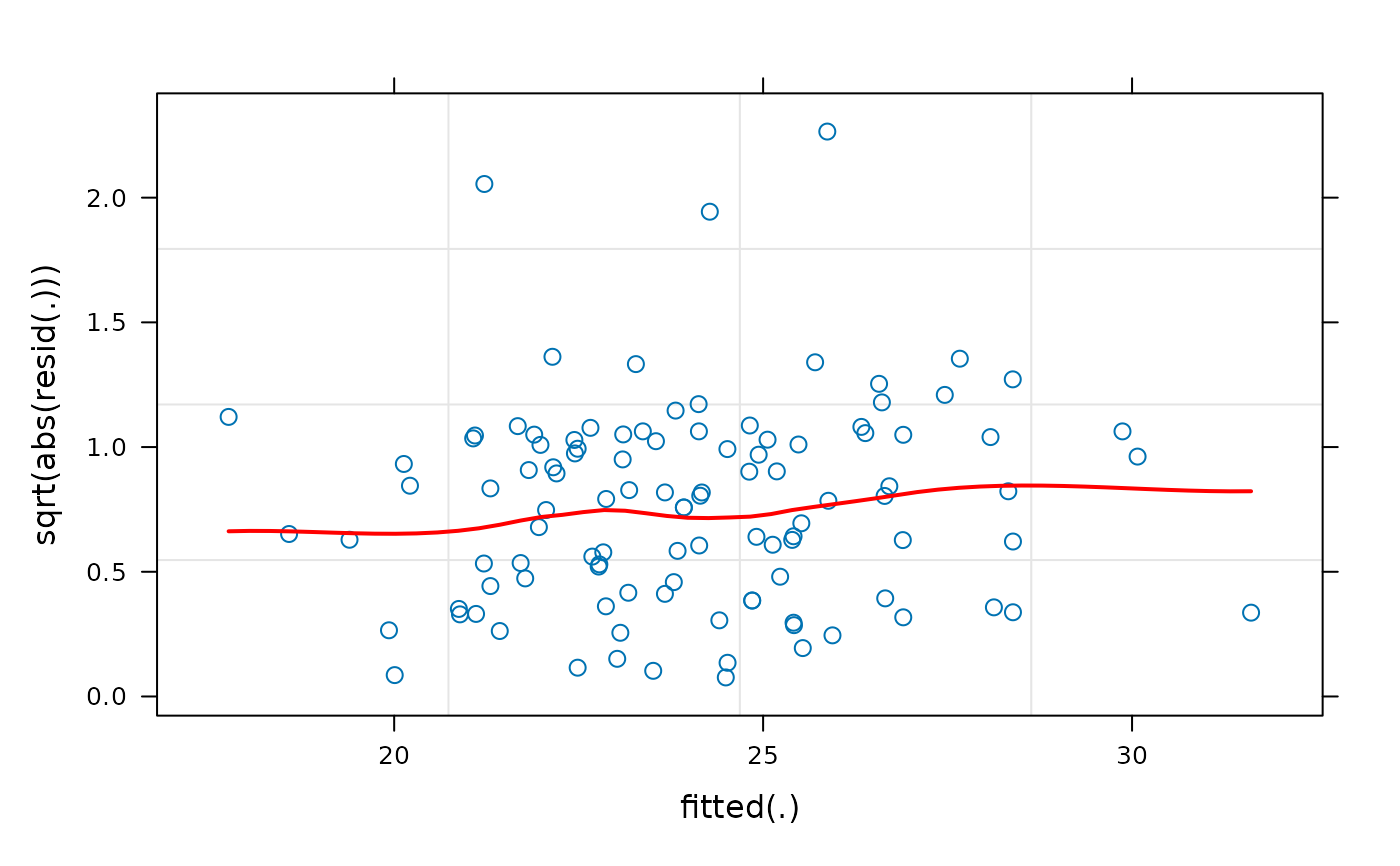
## scale-location plot, with red smoothed line
scale_loc_plot <- function(m, line.col = "red", line.lty = 1,
                           line.lwd = 2) {
  plot(fm1, sqrt(abs(resid(.))) ~ fitted(.),
       type = c("p", "smooth"),
       par.settings = list(plot.line =
                             list(alpha=1, col = line.col,
                                  lty = line.lty, lwd = line.lwd)))
}
scale_loc_plot(fm1)

## Q-Q plot
lattice::qqmath(fm1, id=0.05)

ggp.there <- "package:ggplot2" %in% search()
if (ggp.there || require("ggplot2")) {
    ## we can create the same plots using ggplot2 and the fortify() function
    fm1F <- fortify.merMod(fm1)
    ggplot(fm1F, aes(.fitted, .resid)) + geom_point(colour="blue") +
           facet_grid(. ~ Sex) + geom_hline(yintercept=0)
    ## note: Subjects are ordered by mean distance
    ggplot(fm1F, aes(Subject,.resid)) + geom_boxplot() + coord_flip()
    ggplot(fm1F, aes(.fitted,distance)) + geom_point(colour="blue") +
        facet_wrap(~Subject) +geom_abline(intercept=0,slope=1)
    ggplot(fm1F, aes(age,.resid)) + geom_point(colour="blue") + facet_grid(.~Sex) +
        geom_hline(yintercept=0)+ geom_line(aes(group=Subject),alpha=0.4) +
        geom_smooth(method="loess")
    ## (warnings about loess are due to having only 4 unique x values)
    if(!ggp.there) detach("package:ggplot2")
}
#> Loading required package: ggplot2

Usage

Arguments

Details

See also

Author

Examples